// analysis
Copper: conditions for US stockpiles to return overseas
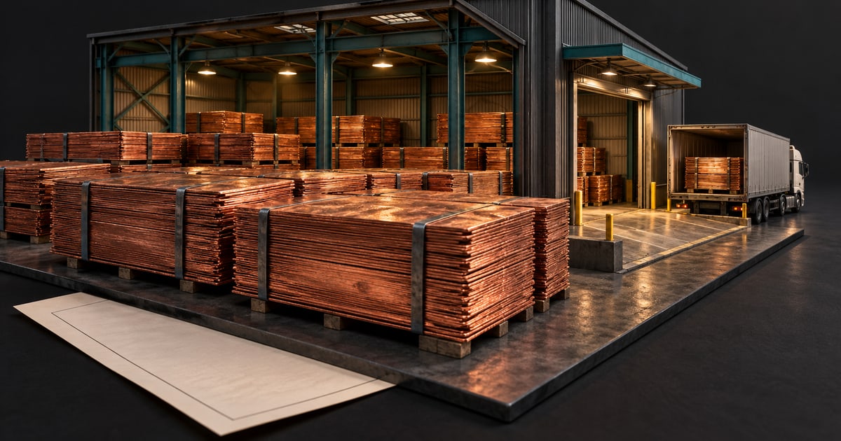
A smaller US premium need not send copper back overseas. Six figures explain the price thresholds, warrants, customs status and physical flows.
On 5 October 2026, a COMEX notice added another location to the copper delivery network: Henry Bath’s warehouse in Laredo, Texas. Its approved capacity is 40,345 US short tons, or approximately 36,600 metric tonnes. Approval makes it a place where metal deliverable against the exchange’s contracts can be stored. The notice establishes neither how full the building is nor when it was built. It does establish another route into the US exchange-delivery system. [1] [4]
Location matters. A manufacturer needs copper it can process. A trader also compares the places where it can sell. The prospect of a customs barrier can alter that second calculation well before any duty is collected. Cargoes change destination, warehouses gain approval and metal settles into a different geography.
In September, l0g examined the carrying costs of this inventory. The next question concerns the reverse journey: what would persuade owners to send US stockpiles to other markets? A narrowing price gap can stop fresh arrivals while leaving existing tonnes exactly where they are. The distinction between halting a flow and unwinding a stock is central to the industrial risk.
A large stockpile with uncertain boundaries
On 14 October, Reuters reported a Macquarie estimate of roughly 1.6 million tonnes of US copper inventory, on and off exchanges. The same report put COMEX stocks above 714,000 tonnes. Two days earlier, a Reuters commentary had cited a Citi estimate of approximately 1.1 million tonnes for the United States. [6] [7]
These totals cannot be read as a forty-eight-hour increase or a statistical confidence interval. We obtained no detailed methodology that would align their observation dates and coverage. The 1.6 million figure therefore remains an attributed estimate. Exchange inventory, metal physically located in a country and the full universe of privately held copper answer different questions.
Warehouse notices offer a firmer foothold. Between late August and early October, three approvals covered copper capacity of 33,565 short tons in Memphis, 44,092 in Chicago and 40,345 in Laredo. Converted into metric tonnes and rounded, these are 30,450, 40,000 and 36,600 tonnes respectively. The figure brings those decisions together without assuming the facilities are full. [1] [2] [3] [4]
Method and scope
Exact conversion: 1 short ton = 0.90718474 metric tonne. Intermediate results rounded to four decimal places: Memphis: 30,449.6558 t; Chicago: 39,999.5896 t; Laredo: 36,600.3683 t. Display rounded to the nearest tonne. These approvals measure neither new construction nor net change across the network. Capacity reductions elsewhere, including Tucson, prevent that inference.
Nor is this selection a net national capacity balance. On 31 August, COMEX also published an approved capacity reduction at 4STOX in Tucson. Reconstructing the entire network would require every change and the preceding capacities. The three approvals support a narrower finding: operators have additional locations at which to receive copper qualifying for exchange delivery. [5]
That qualification gives the metal’s owner another financial exit. The COMEX copper contract requires a specified cathode grade, an approved brand and a designated warehouse. Industrial copper and exchange-deliverable copper are therefore not interchangeable merely because their metal content looks similar. Specifications and documentation help determine the available buyer. [11]
An undecided tariff already influences the destination
The timetable is frequently compressed. Operative clause 7 of the 30 July 2025 proclamation called for a Commerce Department update by 30 June 2026 to determine whether refined-copper duties were warranted: 15% from January 2027, then 30% from January 2028. It set out a decision to be made. As of 14 October, the sources reviewed did not confirm adoption of those rates for refined copper. [8] [6]
Manufactured products fall under a different set of provisions, amended in April and June 2026. Applying one tariff rate indiscriminately to cathodes, wire and equipment containing copper would erase the legal distinctions that determine liability. Those texts are used here to delimit the risk, rather than to recreate the tariff schedule for every product. [9] [10]
Consider the moment when a cargo’s destination is chosen. Buyers who expect a higher future US price relative to other markets may be willing to bid more today. A shipment previously intended for another customer can then become attractive to the US market, provided the gap covers the journey and associated constraints.
One operator may be reducing uncertainty over future supplies. Another may buy physical copper and simultaneously sell a matching futures contract, locking in part of the price difference. A third may retain exposure to the policy decision. All three strategies can produce the same visible event, a warehouse receipt, with very different risks attached. Inventory tonnage does not disclose the positions behind it.
The comparison requires prices that genuinely match: the same unit, admissible quality, consistent dates and known delivery terms. A spread between two screens with different maturities is not automatically an executable return. Transit time, collateral requirements and the ability to complete both legs matter to the operator moving the cargo.
The journey back has a separate threshold
Take a wholly hypothetical example, in dollars per metric tonne. Shipping metal into the United States, together with the other frictions assigned to that transaction, amounts to $300. Moving it in the opposite direction involves $250. Product quality and delivery timing are comparable. Potential tariffs and the option value of waiting for a future decision are excluded.
When the US price exceeds the other market’s price by $600, bringing metal in leaves a $300 advantage after the assumed frictions. If the spread falls to $100, a new import loses its appeal. Yet sending copper already in the United States to the lower-priced market would forgo $100 in sale proceeds and require another $250 for the movement. The exporter would be $350 worse off than by selling locally immediately.
Reversing the arbitrage requires crossing another threshold. In this example, the US price must fall more than $250 below the alternative market’s price. At a spread of −$400, outward shipment offers a $150 advantage. Between −$250 and +$300, neither direction offers a geographic-arbitrage gain in the static model.
Method and scope
Spread d = US price minus other-market price, for comparable quality and dates. Inbound gain = d − 300. Outbound gain relative to an immediate local sale = −d − 250. Break-even thresholds are +300 and −250 $/t. At d = +100, outward gain is −350. At d = −400, it is +150. Duties, option value and contract heterogeneity are not calibrated. Local sales remain possible inside the middle band.
The middle band explains a form of persistence. Incoming cargoes can stop without a symmetrical incentive sending them back out. Existing holders can still sell to US users, transfer ownership or wait. The band indicates the absence of geographic arbitrage under the stated assumptions, not a compulsory freeze on every position.
The original purchase price matters to the owner’s eventual financial result. Choosing between two destinations today turns on the proceeds available and the expenditure still required. Transport already completed is a sunk cost; paying for another journey does not recover it. Losing an earlier opportunity is therefore different from receiving an economic instruction to reverse the shipment.
Policy uncertainty can extend the holding period. In commercial commentary published on 14 September, StoneX discussed the continuing attraction of holding metal in the United States while the refined-copper decision remained open. This market participant’s account illuminates an incentive, without measuring how many owners act on it. The value of waiting depends on contracts, liquidity and expectations that are not publicly observable. [12]
Ownership can move while the cathodes stay put
Exchange delivery introduces another distinction. On COMEX, delivery transfers a warrant, an electronic title to warehoused metal. Its new holder can retain it, sell it or request physical withdrawal. Repeated transactions can consequently concern the same cathodes without the metal leaving the building. [14]
Warehouse reporting distinguishes registered metal, covered by a warrant, from eligible metal that meets the requirements but has no warrant. Receipts and shipments are reported separately. A change of category and a physical movement can therefore be identified as different events. [13]
The figure follows a hypothetical 1,000-tonne parcel. Selling it leaves the total unchanged. Cancelling its warrant and retaining it as eligible stock in this example also leaves the total unchanged. The site’s inventory falls when the tonnes leave. Their destination is still a further fact to establish.
Method and scope
Simplified illustration: 1,000 metric tonnes, no pledged metal, new receipts or subdivision. Stage three assumes the cathodes remain eligible after cancellation. The sequence does not describe every operational case. The final destination remains unknown after exit from this site.
“Off-warrant” does not imply a uniformly invisible universe. The LME has published daily reports covering part of these inventories since April 2025, with public access on a T+3 delay. That reporting does not encompass all privately held metal. What matters is the precise combination of coverage, reporting date, location and status. [15]
For an Asian or European purchaser, a US title transfer may change the counterparty without improving immediate access to copper. A local stock decline becomes more informative once its cause is known: delivery to an industrial customer, transfer to another warehouse or export. A column heading cannot establish a cargo’s route.
Customs status and the applicable duty date
A cargo can be physically inside the United States while remaining in a customs bonded warehouse. The general rule in 19 CFR § 141.69 uses the duty rate in force at entry, subject to exceptions. For merchandise entered for warehousing, it refers to withdrawal for consumption. Specific provisions can override that treatment. [16]
Withdrawal for consumption requires formalities, an estimated-duty deposit and a permit. Unloading, presence in a building and entry for consumption are distinct events. COMEX approval by itself establishes none of the customs records for particular lots that might be stored there. [17]
Method and scope
19 CFR § 141.69 provides exceptions to the general entry rule, including warehousing; § 144.38 governs withdrawal for consumption. A future measure could introduce specific treatment. COMEX approval, a foreign-trade zone and a bonded warehouse are distinct concepts. No aggregate tax advantage is calculated.
It follows that tonnes already on US soil cannot all be assumed to have secured a permanent tax advantage. Establishing that advantage would require their customs status, the relevant date and the provisions of a future measure, should one be adopted. This article therefore makes no calculation of duties supposedly avoided across the aggregate US stockpile.
The distinction also enters the comparison between local sale and shipment abroad. Each operator must use the regime applicable to its own parcel. Two nearby lots can offer different possibilities. Adding their weights provides a physical quantity; it does not harmonise their legal rights or their routes to market.
Leaving the warehouse takes time of its own
An owner with a buyer, an agreed price and the necessary documents still has to load the metal. COMEX Chapter 7 sets out withdrawal procedures. The copper contract, meanwhile, specifies that it carries no freight allowance. Delivering title is therefore different from getting metal to a factory gate. [13] [11]
A 13 October development makes this especially relevant. CME published a notice amending copper load-out procedures. Its summary gives a regulatory effective date of 28 October, pending CFTC review, and operational stages on 1 July 2027 and 1 January 2028. The detailed attachment could not be obtained; no new load-out rate is inferred from the notice’s title. [18]
The economic distinction is straightforward. Inventory is a quantity at a date; loading capacity is a flow over time. One cannot be read directly from the other. Several holders can decide to withdraw at once while appointments, equipment and transport links impose an order on their requests.
This establishes no particular queue in Laredo, Memphis or Chicago. We obtained no loading schedules or measured waiting times. It does identify the missing evidence needed to assess a rapid release: how much metal can actually leave each location and reach its intended buyer within the relevant period? A large inventory with limited throughput provides different protection from the same inventory that can be mobilised quickly.
Hedging the benchmark leaves a delivery exposure
Geographic concentration reaches manufacturers through the price at which they can actually obtain metal. The LME describes physical pricing as a benchmark plus premiums or discounts reflecting such factors as product, location and delivery. A benchmark hedge can leave exposure to those other components. This is basis risk: the thing being purchased does not move exactly like the instrument used to hedge it. [19]
Consider a hypothetical factory planning a purchase at a $10,000-per-tonne benchmark plus a $200 premium. It perfectly hedges the benchmark with a long futures position. By the purchase date, the benchmark falls to $9,500, while the premium rises to $900. The physical invoice is $10,400, compared with the $10,200 initially expected.
The long futures position loses $500, exactly as expected when the benchmark falls. Including the hedge, the purchase requires $10,900. The $700 overrun corresponds entirely to the higher premium. The benchmark hedge has performed its task in this example; access to the locally deliverable product remains exposed.
Method and scope
Initial price: 10,000 + 200 = 10,200 $/t. Final invoice: 9,500 + 900 = 10,400. The long future loses 500, giving a hedged purchase cost of 10,900, or 700 above budget. The contributions sum to −500 +700 +500 = +700. The last bar is the total, not a fourth driver. Matched timing is assumed; fees, financing, taxes and quality differences excluded.
Futures gains and losses are settled daily. Cash outflows on the position may therefore precede payment for the physical parcel. A company must arrange that liquidity even when its hedge makes economic sense. No copper-market margin calls or owners’ losses are estimated here: individual portfolios are unknown. [20] Our investigation into the liquidity required for margin calls examines that funding requirement in energy; it does not quantify copper holders’ positions.
For macroeconomic analysis, transmission is the key issue. A factory may need additional cash, postpone procurement or adjust production while the reference price eases. The response depends on delivery clauses, financial buffers and the ability to pass on changes in purchasing conditions. One price index is a poor description of all those circumstances.
A global balance can coexist with local constraints
The strongest counterargument concerns the value of storage itself. Privately held inventory can secure supplies for nearby users, and delayed deliveries can meet genuine demand tomorrow. A high stock level is not intrinsically a misallocation. Its value depends on the service it provides and the terms on which it can be mobilised.
The global outlook may offer another offset. On 14 October, Reuters reported an ICSG forecast of a refined-copper surplus of 104,000 tonnes in 2026 and 368,000 tonnes in 2027. The full ICSG release was unavailable. These remain attributed forecasts; no geographic breakdown is reconstructed from them. [21]
An annual global surplus describes the expected relationship between production and use. A purchaser of a particular parcel needs another answer: where, when and in what form is metal being offered? New availability can gradually ease premiums and supply pressure. The speed of adjustment also depends on existing inventories returning to circulation.
Even a fall in US stocks would leave room for interpretation. In a final simulation, inventory falls from 200,000 to 180,000 tonnes after receipts of 40,000 tonnes. It could have supplied 60,000 tonnes to US users with no exports. Alternatively, it could have supplied 40,000 tonnes domestically and exported 20,000. The stock decline is identical; the direct effect on supply elsewhere is different.
Method and scope
Two hypothetical scenarios in thousand metric tonnes over the same month. A: 200 + 40 − 60 − 0 = 180. B: 200 + 40 − 40 − 20 = 180. Closed perimeter with no other movements; domestic deliveries are assumed to reach end users. Dashes mark opening stock. Arrows show relationships, not scaled throughput. No actual 2026 stock data are reconstructed.
Advance importing shifts some procurement through time. Once a stockpile has been built, foreign purchases can slow even while factories keep consuming. Conversely, strong imports can fill warehouses without signalling an equivalent acceleration in industrial activity. Our analysis of adjustments in orders and inventories develops this distinction between procurement and use. Measuring these relationships requires observations of use and physical flows.
The next decisive piece of evidence may therefore be less spectacular than the size of the “mountain”. It would combine a price spread consistent with outward shipment, completed physical withdrawals and a verified foreign destination. A lower US premium supplies only part of that evidence. Until the stages line up, the market can stop attracting metal while continuing to retain it.
Sources and scope
Documentary research closed on 14 October 2026. CME notices, COMEX rules, LME explanations and customs provisions were checked alongside market reporting. The three approved capacities are verified against their notices and converted using the NIST factor. They are neither a national census nor an estimate of actual inventory. The Pratima Desai report and Andy Home column were read in full republications by Investing.com (Canada) and Devdiscourse; the original Reuters pages were inaccessible. The COMEX total remains the figure reported by Reuters: CME’s daily inventory workbook could not be retrieved.
Detailed Citi and Macquarie methodologies, individual ownership records, customs statuses and financing contracts were unavailable. The ICSG forecast is reported through Reuters; the CME load-out summary was read without its detailed attachment. No interviews, site visits, cargo tracking or operator audits are claimed. The arbitrage, warrant, hedging and flow illustrations use explicit assumptions. They reconstruct no actual trade and provide no price forecast.
- CME Group / COMEX · 2026-10-05. Regularity Approval for Aluminum, Copper, Lead, and Zinc : Laredo. Notice MKR 10-05-26. Copper capacity approved: 40,345 short tons. Approval is neither measured inventory nor evidence of a newly built facility.
- CME Group / COMEX · 2026-08-28. Regularity Approval for Aluminum, Copper, Lead, and Zinc : Memphis. Notice MKR 08-28-26. Henry Bath, Memphis: 33,565 short tons of approved copper capacity.
- CME Group / COMEX · 2026-09-11. Regularity Approval for Copper : Chicago. Notice MKR 09-11-26. Metal Ox, Chicago: 44,092 short tons. Capacity is distinct from inventory.
- NIST · May 2006; accessed 14 October 2026. SP 1038, The International System of Units (SI): Conversion Factors for General Use. Table 5.2.1, printed page 11: 1 short ton = 2,000 pounds = 0.90718474 metric tonne. l0g conversions rounded to the nearest tonne.
- CME Group / COMEX · 2026-08-31. Approved Decrease in Copper Regularity : Tucson. Approved capacity reduction at 4STOX in Tucson. The three selected approvals cannot be treated as a national net-capacity balance.
- Reuters · Pratima Desai · 2026-10-14. Trump tariff threat built a US copper mountain, but the effects are fading (republication read). Full text read in the Investing.com republication. Macquarie estimate of roughly 1.6 Mt; COMEX stocks above 714,000 tonnes. Detailed methodology and ownership register unavailable.
- Reuters · Andy Home · 2026-10-12. The US has built a strategic copper reserve. Now can it keep it? (republication read). Commentary: Citi estimate of roughly 1.1 Mt. Scope and measurement date are insufficiently documented to reconcile it with Macquarie. Full text read in the Devdiscourse republication; the original Reuters page was inaccessible.
- White House · 2025-07-30. Adjusting Imports of Copper Into the United States. Proclamation 10962, operative clause 7: assessment of possible 15% and 30% refined-copper duties in 2027 and 2028. A contemplated rate is distinct from an applicable decision.
- White House · 2026-04-02. Strengthening Actions Taken to Adjust Imports of Aluminum, Steel, and Copper Into the United States. Amendment to the regime for covered products. No single rate is applied here to all copper.
- White House · 2026-06-01. Further Adjusting the Tariff Regimes for Imports of Aluminum, Steel, and Copper Into the United States. Further 2026 amendment consulted to distinguish covered manufactured products from refined copper.
- COMEX · undated; accessed 14 October 2026. Rulebook, Chapter 111 : Copper Futures. Section 111101, page 1: Grade 1 cathodes, approved brand and warehouse, 25,000-pound contract, no freight allowance. PDF and page examined.
- StoneX · Natalie Scott-Gray · 2026-09-14. Section 232 remains copper’s biggest swing factor into the year-end. Commercial commentary featuring trader Giles Plumb. Informs the holding-incentive discussion; does not measure every owner’s strategy.
- COMEX · undated; accessed 14 October 2026. Rulebook, Chapter 7 : Delivery Facilities and Procedures. 703.A(7) and 703.B, PDF pages 5 and 7–8. Categories, movements and withdrawal. Pledged metal belongs to registered inventory and is not added as a separate stock.
- CME Group · undated; accessed 14 October 2026. What is the Base Metals Delivery Process?. Electronic title transfer, storage, resale or withdrawal request. Educational material from the market operator.
- London Metal Exchange · undated; accessed 14 October 2026. Off-warrant stock reporting. Daily reporting since April 2025; licensed T+1 and public T+3 access. Coverage is distinct from all private inventories.
- eCFR / US Customs and Border Protection · undated; accessed 14 October 2026. 19 CFR § 141.69 : Applicable rates of duty. Read on 14 October; title current through 9 October 2026. General rule and warehouse-entry provision, subject to specific exceptions.
- eCFR / US Customs and Border Protection · undated; accessed 14 October 2026. 19 CFR § 144.38 : Withdrawal for consumption. Consumption-withdrawal formalities, estimated-duty deposit and permit. No particular warehouse’s customs status has been established.
- CME Group / NYMEX–COMEX · 2026-10-13. Amendments to Rule 703.B : Copper Load-Out Procedures. HTML summary read: 28 October regulatory effective date pending CFTC review; operational stages on 1 July 2027 and 1 January 2028. Detailed attachment not obtained.
- London Metal Exchange · undated; accessed 14 October 2026. The role of premiums and discounts in pricing of industrial metals contracts. Reference price, physical premium and basis risk. Figure 5 values are a l0g illustration, not observed prices.
- CME Group · undated; accessed 14 October 2026. Mark-to-Market. Daily settlement of profits and losses. Supports the cash-flow mechanism, not a reconstruction of a real portfolio.
- ICSG, via Reuters / Mining Weekly · 2026-10-14. ICSG sees global refined copper surplus widening in 2027. Forecast: refined surplus of 104,000 tonnes in 2026 and 368,000 in 2027, as reported by Reuters. Full ICSG release unavailable; no global balance recalculated.
This analysis is not investment advice.
// cite this analysis
l0g, “Copper: conditions for US stockpiles to return overseas”, l0g.fr, published October 14, 2026, updated October 14, 2026, https://l0g.fr/en/analysis/copper-us-stockpiles-conditions-for-return/
$ cd ../analysis